Pandas Series

Pandas Series#

This tutorial introduces the fundamental building block of pandas, the Series. By the end of this section, you will learn how to create different types of Series, subset them, modify them, and summarize them.

What is a Series?#

In the simplest terms, a Series is an ordered collection of values, generally all the same type. As examples of what you can do with a series, you can have a Series that contains the ages of everyone in your class (a numeric Series), or a Series of all the names of people in your family (a string Series).

This may sound familiar: isn’t that how we described numpy vectors (i.e. one-dimensional numpy arrays)? Yes! In fact, Series are basically one-dimensional numpy arrays with lots of extra features added on top of them. As we’ll see, almost everything you could do with a numpy array you can do with a Series; Series can just do more. In particular, the Series provides the option to use an explicit index (rather than only using the row numbers), as well as some querying and analysis tools which we’ll discuss through this course.

Series are central to pandas because pandas was designed for statistics, and Series are a perfect way to collect lots of different observations of a variable. We’ll see that the apex of pandas functionality which is found in DataFrames is essentially a collection of Series. Understanding Series will enable you to better understand DataFrames and their value for programming for data science.

Creating a series#

There are lots of ways to create Series, but the easiest is to just pass a list or an array to the pd.Series constructor.

To illustrate, let me tell you about a week at the zoo I wish I owned. Here’s what attendance looked like at my zoo last week:

Day of Week	Attendees
Monday	132 people
Tuesday	94 people
Wednesday	112 people
Thursday	84 people
Friday	254 people
Saturday	322 people
Sunday	472 people

Let’s make a Series for this attendance pattern:

import pandas as pd  # We have to import pandas to use Series!

attendance = pd.Series([132, 94, 112, 84, 254, 322, 472])
attendance

  132
   94
  112
   84
  254
  322
  472
dtype: int64

Indices#

One of the fundamental differences between numpy arrays and Series is that all Series are associated with an index. An index is a set of labels for each observation in a Series. If you don’t specify an index when you create a Series, pandas will create a default index that just labels each row with its initial row number, but you can specify an index if you want. When we explored lists and numpy arrays, we also encountered indices that were used to access individual elements. For 2-dimensional arrays or less, these were essentially the row numbers. These implicit indices of the row numbers are also options in Series, but there’s the option to explicitly label your indices in ways that can make your data easier to analyze.

In the case below, for example, we know that these entries are associated with different days of the week, so let’s specify an index for our attendance Series:

attendance = pd.Series(
    [132, 94, 112, 84, 254, 322, 472],
    index=[
        "Monday",
        "Tuesday",
        "Wednesday",
        "Thursday",
        "Friday",
        "Saturday",
        "Sunday",
    ],
)
attendance

Monday       132
Tuesday       94
Wednesday    112
Thursday      84
Friday       254
Saturday     322
Sunday       472
dtype: int64

Now as we see the rows are labeled with days of the week on the left side, rather than with initial row numbers.

Note that you can always access a Series’ index with the .index property:

attendance.index

Index(['Monday', 'Tuesday', 'Wednesday', 'Thursday', 'Friday', 'Saturday',
       'Sunday'],
      dtype='object')

An important property of index labels is that they stay with each row, even if you sort your data. So if I sort my Series by attendance, not only will rows re-order, but so will the index labels:

attendance = attendance.sort_values()
attendance

Thursday      84
Tuesday       94
Wednesday    112
Monday       132
Friday       254
Saturday     322
Sunday       472
dtype: int64

Note: This seems intuitive with days-of-the-week as our index labels, but it can be confusing when your index starts its life as the default index — the Series’ initial row numbers. For example, if you had not changed our index to be days of the week, then the default index would look like the index labels were just row numbers. But if we then sort the Series, the numbers will shuffle, and they will no longer correspond to row numbers:

attendance = pd.Series([132, 94, 112, 84, 254, 322, 472])
attendance

  132
   94
  112
   84
  254
  322
  472
dtype: int64

attendance = attendance.sort_values()
attendance

   84
   94
  112
  132
  254
  322
  472
dtype: int64

Relationship to `numpy` Arrays#

As you’ve probably noted, there are some similarities in the construction of pandas Series with how we constructed numpy arrays. The biggest difference is the index. In the figure below we can see the code to construct both a numpy array and a pandas Series containing the same entries, however, we can also add a1 explicit index labels that may be easier for us to read or to use to access the row contents. For example, if we were representing financial data for three days of a week: ‘mon’, tue’, and ‘wed’, we may be able to do this as shown in the figure below. Once we’ve created our pandas Series, we can return a numpy array. If b contains a pandas Series, then we can return a numpy array with b.values.

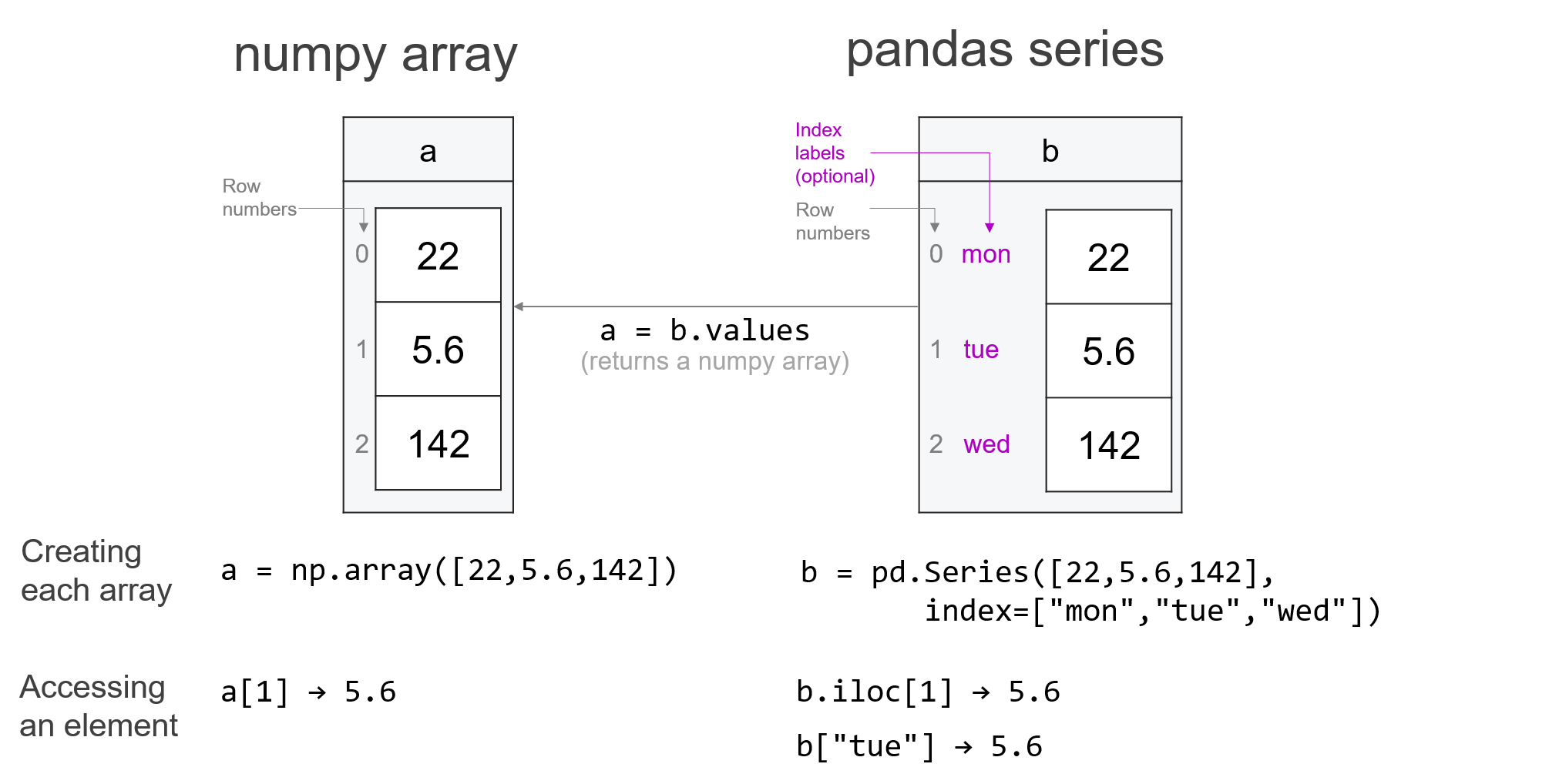
While we will discuss how to access the data in these data structures in more detail in the next lesson, we can rather easily access an entry using the index or its assigned label. There is some nuance in using row numbers since as we saw above with the sort_values() example, the default ordering of row number-based indices can change, so the iloc method will allow us to always return the $i^{th}$ entry regardless of how the Series has been sorted. More on that later, though…

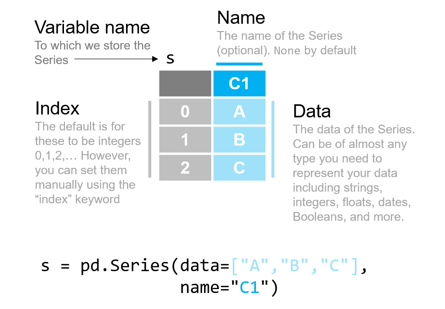
Going forward, we want to be crystal clear when we’re discussing pandas Series or DataFrames instead of when we are talking about numpy arrays. Pictorially, we’ll represent those as little tables as shown below with their key characteristics labeled:

Note: Starting with the release of pandas version 2.0 in 2023, numpy arrays are no longer the only way data can be stored on the back-end by pandas. However, numpy arrays are still the default way data is stored in pandas, so it is what we will use in these lessons. We will discuss the alternate back-end — arrow arrays — added in pandas 2.0 in a future reading.

Types of Series#

Before we dive too far into Series manipulations, it’s important to talk about datatypes. Every Series, as we will see, has a “dtype” (short for datatype). The dtype of a Series is important to understand because a Series’ dtype determines what manipulations you can apply to that series.

There are, broadly, three types of Series:

Numeric: these hold numbers that pandas understands are numbers. Specific numeric datatypes include things like int64, and int32 (integers), or float64 and float32 (floating point numbers).
Object: these are Series that can hold any Python object, like strings, numbers, sets, you name it. They have dtype O for “objects”. They are flexible, but also very slow and actually harder to work with.
Categorical: this is a special data type (analogous to factors in R, if that means anything to you) that we’ll discuss in a future reading. Don’t worry about them for now.

Numeric Series are by far the easiest to work with and are generally either integers (int64, int32, etc.) or floating point numbers (float64, float32). Integer Series (datatypes that start with int) can only hold… well, integers (whole numbers), while floating point numbers Series (datatypes that start with float) can hold integers, numbers with decimal points, and even missing values.

The numbers at the end of these types (64, 32, etc.) have to do with how many actual bits of data are allocated to each number. For the moment, the differences between them don’t matter, and in general, you’ll likely always see (and should use) the 64 suffix.

You can check the dtype of a Series by typing .dtype. For example, here are some different kinds of Series:

s = pd.Series([1, 2, 3])
s.dtype

dtype('int64')

s = pd.Series([1, 2, 3.14])
s.dtype

dtype('float64')

s = pd.Series([1, 2, "a string"])
s.dtype

dtype('O')

As you can see, integer (int64) Series can only hold integers. If we add one number with a decimal component, the whole thing becomes a float64. Similarly, floating point Series can only hold numbers. If we add a single String, the whole thing becomes an Object (O) type.

Converting datatypes#

If you want to change the datatype of a Series, you can do so with the .astype() method… provided a conversion is possible! For example, you can always convert integer arrays to floating point Series because a whole number can be represented as a floating point number (just trust me on this for now… we’ll discuss why later!).

s = pd.Series([1, 2, 3])
s = s.astype("float64")
s

  1.0
  2.0
  3.0
dtype: float64

But be careful: since integers can’t ever hold decimals, if you try and convert a floating point Series to an integer Series, it will just drop the decimal part of numbers with decimals!

s = pd.Series([1, 2, 3.14])
s = s.astype("int64")
s

  1
  2
  3
dtype: int64

Note Pandas is just doing the same thing regular Python would do:

int(3.14)

But if you try and convert an “object” Series to numeric and there are numbers that can’t be converted, pandas will throw an error:

s = pd.Series([1, 2, "a string"])
s.astype('float64')

---------------------------------------------------------------------------
ValueError                                Traceback (most recent call last)
/Users/nce8/github/practicaldatascience/source/10_pandas_series.ipynb Cell 32 in <cell line: 2>()
      1 s = pd.Series([1, 2, "a string"])
----> 2 s.astype('float64')

... 

File ~/opt/miniconda3/lib/python3.10/site-packages/pandas/core/dtypes/cast.py:1181, in astype_nansafe(arr, dtype, copy, skipna)
   1177     raise ValueError(msg)
   1179 if copy or is_object_dtype(arr.dtype) or is_object_dtype(dtype):
   1180     # Explicit copy, or required since NumPy can't view from / to object.
-> 1181     return arr.astype(dtype, copy=True)
   1183 return arr.astype(dtype, copy=copy)

ValueError: could not convert string to float: 'a string'

Computation with Series#

One of the nice things about Series is that, like numpy arrays, we can easily do things like multiply all the values by another number easily. For example, suppose tickets to my zoo cost $15 per person. What is the total money generated by ticket sales each day? Let’s find out!

attendance = pd.Series(
    [132, 94, 112, 84, 254, 322, 472],
    index=[
        "Monday",
        "Tuesday",
        "Wednesday",
        "Thursday",
        "Friday",
        "Saturday",
        "Sunday",
    ],
)
attendance

Monday       132
Tuesday       94
Wednesday    112
Thursday      84
Friday       254
Saturday     322
Sunday       472
dtype: int64

revenue = attendance * 15
revenue

Monday       1980
Tuesday      1410
Wednesday    1680
Thursday     1260
Friday       3810
Saturday     4830
Sunday       7080
dtype: int64

Now what if we want to know the total amount raised in a week, instead of just the amount on each day? We can use one of pandas’s many helper functions — in this case sum — which adds up all the values of a Series:

revenue.sum()

Cool!

This is an example of one of the three forms of Series arithmetic:

Operations involving a Series with more than one element and a single element (like multiplying all values of a Series by 15, as shown above).

Modifying a Series with a function.

revenue**2

Monday        3920400
Tuesday       1988100
Wednesday     2822400
Thursday      1587600
Friday       14516100
Saturday     23328900
Sunday       50126400
dtype: int64

Operations involving two Series. Note that when working with two Series, elements are matched based on index values, not row numbers (the behavior of numpy arrays).

Index Alignment: Matching Entries Using Index Values#

When doing an operation between two Series, pandas matches up entries based not on row number (like numpy or other programming languages like R); rather, it matches up entries based on index values, a practice called index alignment.

This can be a bit tricky, so let’s create a pair of Series to demonstrate:

a = pd.Series(data=[1, 2, 3.2], index=["mon", "tue", "wed"])
a

mon    1.0
tue    2.0
wed    3.2
dtype: float64

b = pd.Series(data=[4.0, 5, 6], index=["tue", "wed", "fri"])
b

tue    4.0
wed    5.0
fri    6.0
dtype: float64

Note that the indices are not the same, although 'tue' and 'wed' are in both Series. Let’s multiply them together:

c = a * b
c

fri     NaN
mon     NaN
tue     8.0
wed    16.0
dtype: float64

Two Series multiplied together that have explicit index labels perform the operation by matching the index values. tue is the second entry in a and the first in b, but pandas matches them up to compute the final entry associated with tue: 2 * 4 = 8.

If an observation has an index value that doesn’t exist in the other Series (e.g., fri and mon), a NaN value is returned.

Of course, with the default row number-based indices, if the data have not been sorted, they multiply element-wise as you would expect:

a = pd.Series(data=[1, 2, 3.2])
a

  1.0
  2.0
  3.2
dtype: float64

b = pd.Series(data=[4.0, 5, 6])
b

  4.0
  5.0
  6.0
dtype: float64

c = a * b
c

   4.0
  10.0
  19.2
dtype: float64

Note that the types of things you can do with a Series depends on the Series dtype. Math functions, for example, can only be applied to numeric datatypes!

Summarizing with Functions#

We often want to get summary statistics from a Series—that is, learn something general about it by looking beyond its constituent elements. If we have a Series in which each element represents a person’s height, we may want to know who the shortest or tallest person is, what the median or mean height is, what the standard deviation is, etc. Here are common summary facts for numeric Series (some also work for object types):

my_numbers = pd.Series([1, 2, 3, 4])

my_numbers.dtype #check the dtype
len(my_numbers) #number of elements 
my_numbers.max() #maximum value
my_numbers.min() #minimum value
my_numbers.sum() #sum of all values in the Series
my_numbers.mean() #mean
my_numbers.median() #median
my_numbers.var() #variance
my_numbers.std() #standard deviation
my_numbers.quantile() #return specified quantile, 0.5 if none specified
my_numbers.describe() #function that contains many summary stats from above
my_numbers.value_counts() # Tabulate out all the values. Add the argument `normalize=True` to get shares in each big. 

Of those, two of the most powerful are .describe() (for numeric Series that take on lots of values):

my_numbers = pd.Series(range(100))
my_numbers.describe()

count    100.000000
mean      49.500000
std       29.011492
min        0.000000
25%       24.750000
50%       49.500000
75%       74.250000
max       99.000000
dtype: float64

and .value_counts() for numeric series with only a few unique values:

my_numbers = pd.Series([1, 2, 2, 2, 2, 1, 1, -1, -1])
my_numbers.value_counts()

 2    4
 1    3
-1    2
Name: count, dtype: int64

Note that .value_counts() can be combined with the normalize=True argument to get the share (i.e. proportion) of observations that have each unique value, rather than the count:

my_numbers.value_counts(normalize=True)

 2    0.444444
 1    0.333333
-1    0.222222
Name: proportion, dtype: float64

Summary#

pandas Series are dynamic tools for representing a wide array of data types than (in general) numpy arrays. While numpy is the preferred tool for highly specialized numerical processing, pandas Series provide an important step towards understanding the representational and querying power of pandas for analyzing tabular data, which is an extremely common and important type of data for data scientists to work with. The Series introduces the idea of labeled and sortable indices which will enhance our ability to query our data. In the next lesson, we will explore how to work with the contents of a pandas Series.