Working with tabular data

Tabular data is any collection of data that can be organized into rows and columns, essentially a two-dimensional matrix, as opposed to unstructured text, network data, geospatial data, image data, and video data, each of which have distinct methods and file formats for the data.

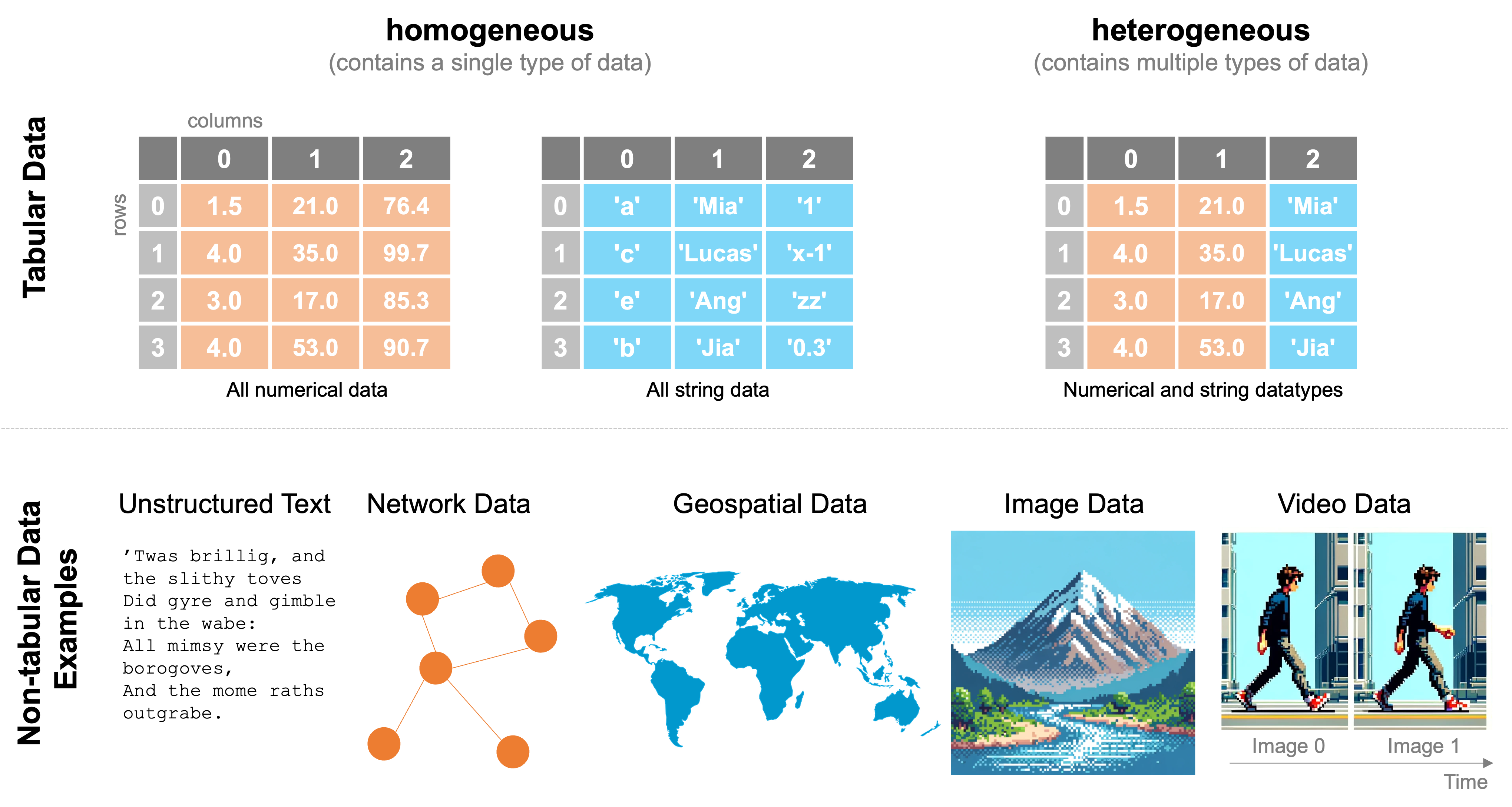
In the last class, we discussed how to work with tabular numerical data through arrays and matrices in cases when all the data were of the same type. You encounter this often, so numpy is a powerful tool for working with such homogeneous data (data of the same type) and in such cases is often the preferred tool if you want to do numeric computations because of its speed. However, there are several frequently encountered situations in which numpy tools may not be ideal and where instead the pandas library may be best. These include:

1. Your data includes not only numerical data, but also text, images, geometric objects, or any other type of data (i.e., your data are heterogeneous). In these situations, numpy may not be appropriate, while pandas can easily organize, manipulate, and analyze this kind of “mixed data.”

2. If you have tabular data — that is, data organized into rows and columns, as in a spreadsheet — it is often easier in pandas to describe, summarize, query, and visualize the data than the equivalent processes with numpy.

Mixed data types

Often our data are of mixed types (e.g. integers and strings). This happens all the time. Imagine that you are collecting basic medical information from a patient. You may ask for height and weight (numerical, floating point numbers), age (integer), and blood type (categorical, string). While numpy can store these together in an array, there’s not much you’re going to be able to do with it computationally. Consider the following example where numpy throws an error:

import numpy as np
a = np.array([6.1,150.0,25,'A-'])
b = np.array([5.6,122.0,29,'B+'])
c = a + b

---------------------------------------------------------------------------
UFuncTypeError                            Traceback (most recent call last)
c:\Users\kjb17\Dropbox\Code\mids_coursera\class_3\week_2\10_intro_to_pandas.ipynb Cell 2' in <module>
      2 a = np.array([6.1,150.0,25,'A-'])
      3 b = np.array([5.6,122.0,29,'B+'])
----> 4 c = a + b

UFuncTypeError: ufunc 'add' did not contain a loop with signature matching types (dtype('<U32'), dtype('<U32')) -> None

pandas, on the other hand, doesn’t have any problem with mixed data types. It will use the appropriate operation for each data type, adding the numbers and concatenating the strings:

import pandas as pd

a = pd.Series([6.1, 150.0, 25, "A-"])
b = pd.Series([5.6, 122.0, 29, "B+"])
c = a + b
c

0     11.7
1    272.0
2       54
3     A-B+
dtype: object

In the summer of 2023, the pandas package was updated to pandas 2.0. In most cases, pandas 2.0 operates in the same manner as pandas 1.0, but there are a few important differences. All materials in this course reflect the behavior of pandas 2.0, and where the behavior of pandas 2.0 is notably different from the behavior of previous versions of pandas, we will note that explicitly.

It is important you understand this change took place recently because the various versions of pandas 1.x (e.g., pandas 1.0, 1.1, 1.2, ...) were around for over three years, and much of the behavior of pandas 1.x was also present before pandas 1.0 was released. As a result, a lot of answers you find on resources like StackOverflow or Google, or code you get from generative AI tools like chatGPT or Github Copilot will be based on behavior that, in places, may now be out of date!

A hierarchy of data types: from lists to numpy arrays to pandas Series and DataFrames

In this section, we’re introducing pandas objects/data types including the Series and the DataFrames.

We can think of a pandas Series as a 1-dimensional numpy array with more functionality for selecting and querying data than we get in a 1-dimensional numpy array. DataFrames, similarly, are a collection of Series analogous to a 2-D numpy array, but with even more querying tools built into the objects themselves.

Effectively working with tabular data

Let’s walk through 3 examples of what you can do easily with pandas that can be rather complicated without it:

1. Quickly reading your data into a structured tabular form

2. Quickly describe/summarize your data

3. Quickly querying your dataset

4. Quickly plotting your data

Example 1: Quickly reading your data into a structured tabular form

Using the convenient pandas methods that hide away the tricky bits, loading tabular data is trivially easy. Let’s load in a dataset to demonstrate (we’ll talk more about how these work throughout this week):

import pandas as pd

smallworld = pd.read_csv("./data/world-very-small.csv")
smallworld

	country	region	gdp_per_capita_2008
0	Brazil	S. America	10296
1	Germany	W. Europe	35613
2	Mexico	N. America	14495
3	Mozambique	Africa	855
4	Russia	C&E Europe	16139
5	Ukraine	C&E Europe	7271

It really doesn’t get much easier than that. We have text content (under country and region) and numerical content (`gdp_per_capita_2008``) and column headings are even included!

Example 2: Quickly describe / summarize your data

With the use of a single pandas method, we can summarize the statistics of any fully-numerical columns of data:

smallworld.describe()

	gdp_per_capita_2008
count	6.000000
mean	14111.500000
std	11863.031683
min	855.000000
25%	8027.250000
50%	12395.500000
75%	15728.000000
max	35613.000000

Example 3 Quickly querying your data

Not only can we load and describe our data quickly, but we can query our data quickly, too. Let’s say we wanted to find the countries on the list with per-capita GDP below $10,000. This also becomes extremely simple:

smallworld.loc[smallworld.gdp_per_capita_2008 < 10000]

	country	region	gdp_per_capita_2008
3	Mozambique	Africa	855
5	Ukraine	C&E Europe	7271

Example 4: Quickly plotting your data

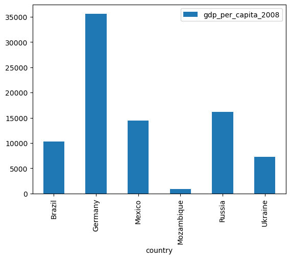
If you want/need a quick look at your data, plotting is extremely straightforward with pandas, as it builds on the matplotlib ecosystem for plotting. Let’s create a bar plot of the GDP per capita for each of the countries in our list:

smallworld.plot.bar(x="country", y="gdp_per_capita_2008")

<Axes: xlabel='country'>

Drawbacks of pandas

Despite its many advantages, and as with all tools, pandas also has its drawbacks. First of all, the syntax of pandas is a bit different from what we’ve discussed previously with base Python and with numpy, making it a bit challenging to learn. Personally, I still find myself regularly consulting the documentation for pandas when I’m using a method I haven’t used in a while. The other drawback is that pandas is particularly well-designed for 1D series/arrays and 2D matrices. It’s not suitable for handling 3D or N-D matrices (where N > 3). In such cases, there are two main options. The first is to simply revert to our trustworthy friend numpy — it’s extremely flexible, powerful, and you already know how to use it! The second option is to use the xarray package, which is to higher-dimensional numpy arrays what pandas is to 1 or 2D numpy arrays — essentially a wrapper around numpy arrays that adds an ability to label your dimensions in a more intuitive manner!

The week ahead

With a sense of the benefits of pandas, this week we will dive into how pandas can be effectively deployed as a key programming tool in working with tabular data and used to construct targeted, and sometimes complicated, queries of tabular data that can be used to answer key data science questions.