Welcome to Matrices#
In the last module of this course, you are introduced to the numpy library, the backbone of data science computing in Python. In particular, we introduced you to numpy vectors, the most basic flavor of the numpy array. We talked about why vectors are useful for data science—when doing science, we usually have lots of measurements of the same property, so it makes sense to collect those in a vector—and why we use numpy instead of vanilla Python data structures like lists (speed, speed, speed!). In addition, we talked about how to do math with full vectors of data in a very concise manner, as well as how we can subset vectors and make modifications to parts of vectors.
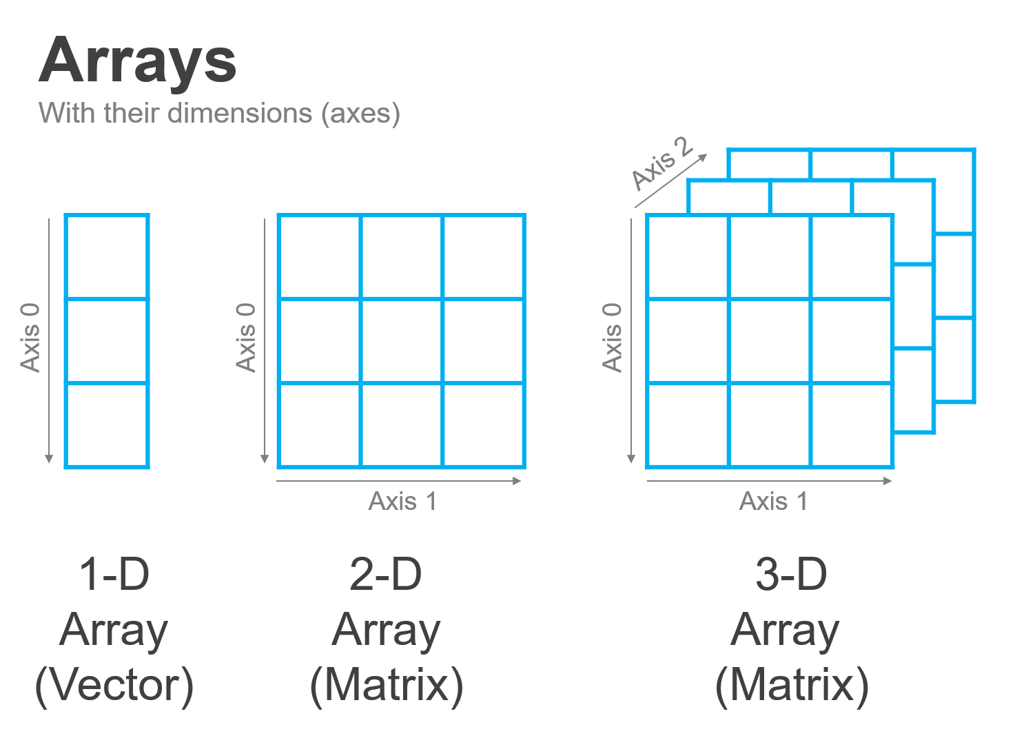
As you may recall from our introduction of vectors, however, vectors are only the simplest implementation of a numpy array— the case when data is only laid out along a single dimension. But numpy arrays come in many different flavors depending on the number of dimensions along which data may be organized, as illustrated below:
Our focus in Week 3 will primarily be on how the approaches for working with vectors that we learned in Week 2 will generalize to other types of numpy arrays. After a quick digression into one of the nuances of vectors we didn’t have a chance to address last week, we will turn our attention to matrices—numpy arrays that arrange data along two dimensions in a grid. As we will see, everything we learned about vectors will generalize naturally as we move from one dimension to two, allowing us to leverage the work we did last week to dramatically increase the types of data manipulations we are able to accomplish.
So as we move forward, remember that our transition from vectors to matrices—and then to arrays with more than two dimensions—is not really a change in subjects, but rather a continued evolution in our understanding of how to work with numpy arrays.